Power Spectrum Measurement¶

If you are looking for a very simple way to measure the power spectral density of a received signal with the AIR-T, you may like the Soapy Power Project. Soapy Power is a part of the larger SoapySDR ecosystem that has built-in support on the AIR-T. In this post, we will walk you through the installation of Soapy Power on the AIR-T and provide a brief demo to help get you started.

Requirements¶

• Artificial Intelligence Radio Transceiver (AIR-T)
• AirStack 0.4.0+
• Internet connection (for install only)

Installation¶

1. Follow the instructions in this tutorial to create the airstack conda environment. We will be using this as the base environemnt and install a few more python packages on top of it. Once the environment is created, activate it per the instructions in that tutorial.

2. Install the cython package first:

   pip install cython
   

3. Install the following 4 packages:

   pip install simplesoapy simplespectral soapy_power pyfftw
   

4. The AIR-T's driver for Soapy is "SoapyAIRT". To verify that your devices is connected, and the installation was successful, execute the following in the terminal:

   python -c "import simplesoapy; print(simplesoapy.detect_devices(as_string=True))"
   

   which will return:

   ['driver=SoapyAIRT']
   

Take a Spectrum Using the AIR-T¶

Using Soapy Power, it is very easy to acquire a spectrum snapshot and record to a csv file. Sample rate, center frequency, and processing parameters can all be controlled via command-line arguments as you will see in the below example.

Please refer to the Installation section below to add the soapy_power tool to your AIR-T, then keep reading to see how to use it to collect and visualize data.

Activate the airstack conda environment:

conda activate airstack

soapy_power -g 0 -r 125M -f 2.4G -b 8192 -O data.csv

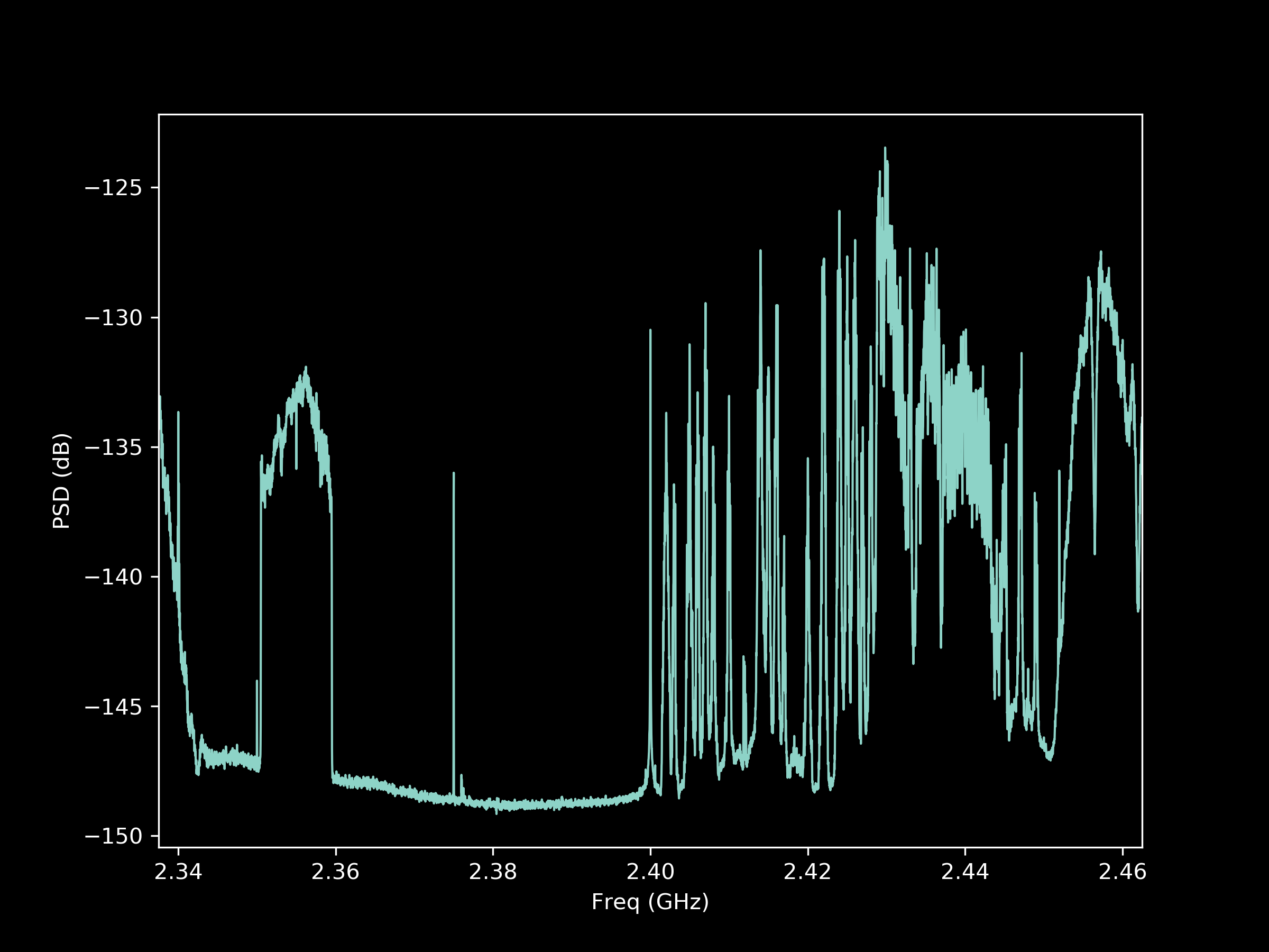
Let's walk through this command. The soapy_power command is the program being called. the -g 0 option sets the gain to 0 dB. The -r 125M option sets the receiver sample rate to 125 MSPS. The -f 2.4G option tunes the radio to 2.4 GHz frequency. We set the FFT size to be 8192 samples using the -b 8192 and average 100 windows using the -n 100 option. Finally, the output file is defined by the -O data.csv option. Following the execution of the above command, a file is recorded with the spectrum data.

To visualize the data, we will use Python's matplotlib package with the following script:

#!/usr/bin/env python3

import numpy as np
from matplotlib import pyplot as plt

with open('data.csv', 'r') as csvfile:
    data_str = csvfile.read()  # Read the data
data = data_str.split(',')  # Use comma as the delimiter

timestamp = data[0] + data[1]  # Timestamp as YYYY-MM-DD hhh:mmm:ss
f0 = float(data[2])  # Start Frequency
f1 = float(data[3])  # Stop Frequency
df = float(data[4])  # Frequency Spacing
sig = np.array(data[6:], dtype=float)   # Signal data
freq = np.arange(f0, f1, df) / 1e9  # Frequency Array

# Plot the data
plt.plot(freq, sig)
plt.xlim([freq[0], freq[-1]])
plt.ylabel('PSD (dB)')
plt.xlabel('Freq (GHz)')
plt.show()

Resulting Power Spectral Density Plot¶