CUDA Blocks with GNU Radio and the AIR-T
This tutorial will teach you how to integrate GPU processing using CUDA with GNU Radio on the AIR-T software defined radio. Once completed, you will be able to build a custom GPU processing block within GNU Radio and use it to process your own signals. The tutorial assumes some familiarity in programming in Python and writing GPU kernels using CUDA. Don't worry if you have never written a GNU Radio block before, this part is explained for you and you can start by modifying the code in the tutorial's GitHub repository to get a feel for how all the components fit together.
Note: This tutorial was written for AirStack 0.3.0 to 0.4.2 and will likely not work yet for versions newer than 0.4.2.
Overview
The below sections will walk you through how to create a very simple GNU Radio block in Python that executes on the GPU. This simple block will use the PyCUDA library to divide the input signal by two and send the result to the output. All computation within the block will be done on the GPU. It is meant to be a very simple framework to understand the process of developing signal processing code.
Note that this tutorial documents software APIs that may change over time. In all of the below examples, we will be working with GNU Radio 3.7.9 (as released with Ubuntu 16.04 LTS) and developing blocks using Python 2.7.
For the impatient, here is the source code.
Introduction
Before beginning, it is important to have some knowledge regarding GNU Radio’s mechanism for “Out of Tree” or “OOT” modules. This allows the author of a signal processing block to build their block in its own repository as a module and then load it into an installed copy of GNU Radio. An in depth tutorial on how to build your own OOT module (this process was used to develop the example code in this tutorial) can be found here: https://wiki.gnuradio.org/index.php/Guided_Tutorial_GNU_Radio_in_Python. It is highly recommended to complete the Python GNU Radio tutorial before proceeding with this tutorial.
In addition to some knowledge with GNU Radio, this document also assumes that you have some background with GPU processing using CUDA.
It should be noted that the scope of this tutorial is to integrate a custom CUDA kernel with GNU Radio, which may not be the right way to solve your problem. NVIDIA also provides “higher level” APIs such as cuFFT (for Fourier transforms) and cuBLAS (for linear algebra). Your application may benefit with interfacing with these APIs directly instead. If you require FFTs run on the GPU via cuFFT, check out the FFT block in gr-wavelearner. Another option is to write your own code to tie these libraries into GNU Radio. If you need to go down this path, you can certainly follow the excellent GNU Radio OOT tutorial for Python (referenced earlier) or the one for C++. However, if you require a custom CUDA kernel to do your processing, then this is the correct tutorial for you.
A final caveat is that our approach here is to use Python as much as possible, as the language lends itself well to rapid prototyping and development (thus decreasing time to market). However, there is a non-trivial performance cost associated with using Python. Whether or not that cost matters for your particular application is a question only repeated benchmarking of your code can answer. That said, GNU Radio and PyCUDA (a Python interface to CUDA, which we use in this example) all use C/C++ underneath and are generally just Python wrappers on top of compiled and optimized code. However, there still is a cost with regards to the Python interpreter being used to access the C/C++ code underneath. For most applications, this cost is negligible and well worth the benefits of working in Python, but once again, you should benchmark and profile your code to see if this cost matters to you. Based on the complexity of your CUDA kernel, you may be pleasantly surprised at the profiling results.
Getting the Source Code
Source code for this example can be found at the Deepwave Digital GitHub page. The README at the top level of this GitHub repository provides instructions on how to get the GNU Radio module (named gr-cuda) installed. This module provides the basic design for integrating CUDA processing with GNU Radio and we will be exploring this design and demonstrating how to modify it in this tutorial. The repository also contains an example GNU Radio flowgraph to execute the new module, as shown below.
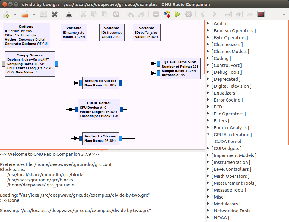
Note that you can validate the gr-cuda install by opening up GNU Radio Companion. On the right side of the window, where blocks are listed, you should see a category entitled “GPU Acceleration”. Within that category you should see a block labeled “CUDA Kernel”. If this block is present, the installation was a success.
GNU Radio Companion Examples
Now that the gr-cuda module is installed, you can run some example flowgraphs. There are three flowgraphs available for testing in the test/ subdirectory. The first two files of interest are complex_constant_src_test.grc and constant_src_test.grc. Both of these flowgraphs simply take a constant input (note that one flowgraph handles complex input, while another is just “standard” floats), samples it, and then runs it through the CUDA kernel before writing the output to a file (found in the test/ subdirectory, and labeled “data.dat”). A final flowgraph, constant_src_rate_test.grc, is useful for benchmarking the rate at which non-complex samples are processed by the CUDA kernel. It does not write the output to a file, since file operations can bottleneck the flowgraph. In the example CUDA block, the kernel is written to simply take every sample and divide it by two, so your output file should be full of samples which are all half of the input samples. Feel free to familiarize yourself with the flowgraphs and the CUDA Kernel block (the block's “documentation” tab is especially useful as it contains information regarding the block’s various parameters).
One particularly important concept in the example flowgraphs is the fact that there is one CUDA kernel block per flowgraph. This is done because data in GNU Radio is passed between blocks via buffers that reside on the CPU. As a result, for each CUDA block, you need to do a transfer between the CPU and GPU each time data arrives at the block. Also, a GPU to CPU transfer must take place as data leaves the block. So, in order to minimize the number of transfers between CPU and GPU (which are a performance bottleneck for most GPGPU applications), it is better (and easier to follow) to have one complex kernel block instead of several smaller blocks that each do a specific function. Note that it is possible to have two adjacent GPU processing blocks and for them to share data on the GPU between one another (i.e., by sending a device pointer as a message to the next block). However, this can make the flowgraph somewhat difficult to follow. Also, such blocks are more difficult to implement with regards to their interface to GNU Radio. Therefore, as a best practice, it is easiest to simply have one GPU processing block per flowgraph that does all the necessary processing on the GPU.
Another key concept in the flowgraphs is the fact that a “Stream to Vector” block comes directly before the CUDA Kernel block. GPUs perform best when handed large amounts of data that can be processed in parallel. In order to achieve this, a “Stream to Vector” block is used to buffer a large number of samples (the flowgraphs default to 131072 samples) before passing this data to the GPU. While this buffering does induce some additional latency, the end goal of our CUDA kernel is throughput, which is maximized by these buffering operations. It should be noted that our block is architected with this in mind (i.e., that it will receive one or more vectors of samples and then process a vector’s worth of samples at a time). Another way of accomplishing the same net effect (that may increase performance in certain cases) is to simply design the block to receive a stream of samples and then to pass the number of samples processed for each kernel invocation to self.set_output_multiple() in the block’s initialization routine. This eliminates the need for a “Stream to Vector” block, since the GNU Radio scheduler is simply told to always pass a certain multiple of samples to our block. However, it has been shown experimentally that this alternative approach can decrease performance and does increase code complexity somewhat, since the programmer no longer has the useful abstraction of knowing that a vector will be processed for each invocation of the CUDA kernel.
Code Deep Dive, Part 1: XML Block Description
Now that you have familiarized yourself with the example flowgraphs, let’s dive into the code that implements the "CUDA Kernel" block. This is what you will need to modify to implement your own GPU-based algorithm.
First, it’s important to note that the directory structure you see in the gr-cuda repository was automatically generated by a utility called gr_modtool. This utility is part of GNU Radio and was written specifically to help authors of new processing blocks get started. It will create both the boilerplate for the GNU Radio module as well as an empty block into which signal processing code is inserted. Note that the block that was created for this example was a “sync” block type, which creates a single output sample for each input sample. Many signal processing blocks follow this form, but if this is not the case for your application, you will more than likely need to run gr_modtool yourself in order to create the “skeleton” code for your particular block type (you will still be able to reuse a good amount of the gr-cuda code, however). Details regarding block types can be found in the previously mentioned GNU Radio tutorials.
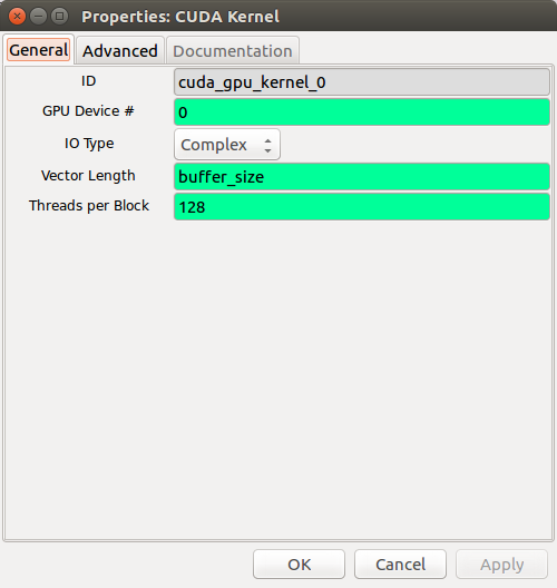
Once gr_modtool created the directory structure for us, only two files were modified for our needs. The first is an XML file that describes the block to GNU Radio Companion. In effect, this will create the image above when opening the block in GNU Radio Companion. This code is found in the grc/ subdirectory and the file is named cuda_gpu_kernel.xml. Open the file so that we can inspect it further. Near the top of the file you will see the following:
 <name>CUDA Kernel</name>
 <key>cuda_gpu_kernel</key>
 <category>GPU Acceleration</category>
 <import>import cuda</import>
 <import>import numpy</import>
 <make>cuda.gpu_kernel($device_num, $io_type.dtype, $vlen, $threads_per_block)</make>
Here the “name” tag references the name that the block will be called in GNU Radio Companion. The “key” is a unique key for the block, so GNU Radio Companion knows which block this is. The “category” tag is the category that the block is listed under in GNU Radio Companion (i.e., at the right hand side of the main window). The two “import” tags are used to import external Python libraries when generating the top_block.py script. In this case, we need the “cuda” library (which is the name of our OOT module) and the “numpy” library since we will be dealing with numpy arrays. Finally, the “make” tag specifies how the block’s init() function gets called when the top_block.py script is generated. In this case, we pass in parameters that are set within GNU Radio Companion. The next chunk of code (shown below) describes how these parameters can be modified by the user.
 <param>
  <name>GPU Device #</name>
  <key>device_num</key>
  <value>0</value>
  <type>int</type>
 </param>
 <param>
  <name>IO Type</name>
  <key>io_type</key>
  <type>enum</type>
  <option>
   <name>Complex</name>
   <key>complex</key>
   <opt>dtype:numpy.complex64</opt>
  </option>
  <option>
   <name>Float</name>
   <key>float</key>
   <opt>dtype:numpy.float32</opt>
  </option>
 </param>
 <param>
  <name>Vector Length</name>
  <key>vlen</key>
  <value>1</value>
  <type>int</type>
 </param>
 <param>
  <name>Threads per Block</name>
  <key>threads_per_block</key>
  <value>128</value>
  <type>int</type>
 </param>
Note that each of these parameters is described in detail in terms of how they affect the block in the block’s documentation tab in GNU Radio Companion. What’s important to understand from the code, however, is how each parameter has a “key” associated with it, which can be thought of as a unique variable name which we can use to pass the parameter around (like in the “make” tag). Each parameter also has a “value” associated with it which is its default value. Finally, each parameter has a “type” associated with it (“int”, “string”, etc.).
The one special case in these parameters is the “IO Type” parameter, which allows us to handle either complex or non-complex sample types. Namely, this is an “enum” type, which will cause GNU Radio Companion to create a dropdown menu for us with the options we list. By default, the first listed option will be selected when the block is created. Note that each option in the enumeration has its own key, which can be passed around as a parameter. We also create an “opt” option for each of the enumerated values. Namely, we create a “dtype” option, which allows us to directly pass the numpy type associated with complex or non-complex data. This lets us pass in “io_type.dtype” to the “make” tag, which will in turn pass the correct numpy type to our block’s init() function.
The next block of code simply allows us to check if the user passed in sane values before generating the top block. In our case, we are simply checking to see if the vector length and number of threads per block are both greater than zero. In general, it is difficult to build complex error handling schemes from within this XML file, but these checks are useful because the block will indicate errors to the user in GNU Radio Companion, well before the flowgraph is executed.
 <check>$vlen > 0</check>
 <check>$threads_per_block > 0</check>
Finally, we have XML code to describe the inputs (i.e., “sinks”) and outputs (i.e., “sources”) of the block. For the CUDA Kernel block, we have one input and one output port as shown in the code below.
 <sink>
  <name>in</name>
  <type>$io_type</type>
  <vlen>$vlen</vlen>
 </sink>

 <source>
  <name>out</name>
  <type>$io_type</type>
  <vlen>$vlen</vlen>
 </source>
Note that for each “type” and “vlen” tag, we pass in values from the parameters passed in by the user. This allows the block to dynamically update itself as the user is changing the vector length or the type of data we are processing.
Code Deep Dive, Part 2: Python GNU Radio Block
The second file of importance in the repository is found in the /python folder, entitled gpu_kernel.py. When we created the block, we had gr_modtool create a Python block for us to use, since we can bring in CUDA processing via the PyCUDA library. This saves much development time versus creating a C++ block and then needing to link in CUDA code. Also, in terms of performance, PyCUDA has been shown to perform at about 80% the throughput of native CUDA code, which is sufficient for most applications.
The first part of the source code creates and documents the gpu_kernel class. Note that this documentation is what GNU Radio Companion uses in the documentation tab of the block. For the purposes of this document, the entire text blob is excluded below. However, it is important to note that the documentation text should contain “run on” lines (i.e., the developer should not insert line feeds to clean up the text blob in the code) to allow for the text to be properly formatted in GNU Radio Companion. Also, note that the block can alternatively be documented via a “doc” tag in the previously mentioned XML file (there are several examples of this approach in the GNU Radio source code).
class gpu_kernel(gr.sync_block):
 """
  <DOCUMENTATION GOES HERE>
 """
The first method in the class is the init() method, which initializes the block and also allocates several GPU resources. It's important to note that this method will be called by GNU Radio once, so it is a good place to pre-allocate resources that can be used over and over again when the block is running. The first thing we do in the init() function is to call the parent class’s init() function. In our case, this is a sync block, since our block has a single output sample for every input sample. Also, note that we pass both the io_type and vlen parameters (both of which are set by the user) for both our input and output signature. This tells GNU Radio that our block’s input and output is a buffer of type io_type and of length vlen.
 def __init__(self, device_num, io_type, vlen, threads_per_block):
  gr.sync_block.__init__(self,
   name = "gpu_kernel",
   in_sig = [(io_type, vlen)],
   out_sig = [(io_type, vlen)])
Next, we initialize PyCUDA. The instance of the class maintains a copy of the context so that we can access the context again when the work() method is called. Note that we edit the context flags (by default only the SCHED_AUTO flag is present) such that the MAP_HOST flag is passed in. This is a critical step since we will be using device mapped pinned memory (which results in a zero copy on embedded GPUs such as the Jetson TX2). Setting the context flags can be skipped if you are using a different CUDA memory API. We then build the device context with these flags. This is necessary since in GNU Radio each block is given its own thread. Therefore, in order to share a GPU between multiple blocks (and therefore threads), we have to create a new device context for each block we create, and then push/pop that context as necessary. More information concerning multithreading in PyCUDA can be found here.
  # Initialize PyCUDA stuff...
  pycuda.driver.init()
  device = pycuda.driver.Device(device_num)
  context_flags = \
   (pycuda.driver.ctx_flags.SCHED_AUTO | pycuda.driver.ctx_flags.MAP_HOST)
  self.context = device.make_context(context_flags)
Now that we have PyCUDA initialized, we can build our kernel. In our case, we have a simple kernel that just divides every input by two and writes the result to the output. Note that this could have been further optimized to do the division in place (i.e., by just writing the result back into the input buffer), but the objective here is primarily to understand the “plumbing” between CUDA inputs and outputs to GNU Radio inputs and outputs. Here we chose to write the kernel inside of the Python file, but if you wish, you can also import a compiled CUDA kernel by calling pycuda.driver.module_from_file() instead of the module_from_buffer() call that we are using. In our case, we are actually compiling the CUDA kernel inside our init() function, which could slow down initialization somewhat, but will not affect the block’s overall runtime.
  # Build the kernel here. Alternatively, we could have compiled the kernel
  # beforehand with nvcc, and simply passed in a path to the executable code.
  compiled_cuda = pycuda.compiler.compile("""
   // Simple kernel that takes every input and divides by two
   __global__ void divide_by_two(const float* const in,
                  float* const out,
                  const size_t num_floats) {
    static const float kDivideByMe = 2.0;
    const int i = threadIdx.x + (blockIdx.x * blockDim.x);
    if (i < num_floats) {
     out[i] = in[i] / kDivideByMe;
    }
   }
  """)
  module = pycuda.driver.module_from_buffer(compiled_cuda)
With the module created and the kernel compiled, the next lines of code in init() extract the kernel function from the compiled code. Note that we use the PyCUDA API to “prepare” the call, which saves us the overhead of having to determine the parameter type each time the kernel is launched. Also, we keep track of how many threads there are in a block, since this will become important when we launch the kernel.
  self.kernel = module.get_function("divide_by_two").prepare(["P", "P", "q"])
  self.threads_per_block = threads_per_block
Finally, after saving off the type of samples we are handling in an instance variable, we allocate device mapped pinned memory using another method that we have written. We are using this type of memory because it provides the best performance on embedded GPUs such as the Jetson TX2, where physical memory for the CPU and GPU are one and the same. For PCIe based cards, it is recommended to use the unified/managed memory API (more details here). We allocate memory in the init() function because we want to avoid having to allocate memory when the block is actually running, which would slow down our block considerably. Note that we allocate enough memory for vlen samples, since our block is designed to process a vector’s worth of samples for each kernel invocation. Also, note that the last line of code cleans up the device context.
  # Allocate device mapped pinned memory
  self.sample_type = io_type
  self.mapped_host_malloc(vlen)
  self.context.pop()
The next method, entitled mapped_host_malloc(), in the gpu_kernel class takes care of device mapped pinned memory allocation. First, the appropriate PyCUDA function is called to allocate and zero fill memory on the host (for both the input and output buffers). The next two PyCUDA calls take the host memory and extract a pointer to device memory from it. Note that this last step is specific to device mapped pinned memory which, as discussed previously, was chosen due to its superior performance on embedded GPUs such as the Jetson TX2.
 def mapped_host_malloc(self, num_samples):
  self.mapped_host_input = \
   pycuda.driver.pagelocked_zeros(
    num_samples,
    self.sample_type,
    mem_flags = pycuda.driver.host_alloc_flags.DEVICEMAP)
  self.mapped_host_output = \
   pycuda.driver.pagelocked_zeros(
    num_samples,
    self.sample_type,
    mem_flags = pycuda.driver.host_alloc_flags.DEVICEMAP)
  self.mapped_gpu_input = self.mapped_host_input.base.get_device_pointer()
  self.mapped_gpu_output = self.mapped_host_output.base.get_device_pointer()
Next, the mapped_host_malloc() function saves the number of samples in an instance variable. After that, we figure out the number of floats we are computing for each kernel invocation. Since our kernel operates on 32-bit floating point values, we need to handle the case of complex data, where we have two of these data types for every sample. As a result, num_floats can either be equal to num_samples (in the case of non-complex data) or twice as large as num_samples (in the case of complex data).
  self.num_samples = num_samples;
  self.num_floats = self.num_samples;
  if (self.sample_type == numpy.complex64):
   # If we're processing complex data, we have two floats for every sample...
   self.num_floats *= 2
The final steps of the mapped_host_malloc() method involve computing the grid and block dimensions for the CUDA kernel. Since we are performing the computation only in one dimension, this greatly simplifies the calculation of these dimensions. Namely, all we do is take the number of floats we have to process and divide by threads_per_block (which is set by the user in GNU Radio Companion). If these numbers are not an even multiple of one another, we simply add another block so that all samples can be processed. Note that the CUDA kernel is written to account for this fact as well, and will not process more than num_floats items per kernel launch (i.e., in the case where num_floats is not an even multiple of threads_per_block, the last thread block will have some threads not perform the computation since doing so would step outside the boundaries of the input and output buffers).
  self.num_blocks = self.num_floats / self.threads_per_block
  left_over_samples = self.num_floats % self.threads_per_block
  if (left_over_samples != 0):
   # If vector length is not an even multiple of the number of threads in a
   # block, we need to add another block to process the "leftover" samples.
   self.num_blocks += 1
The next method in the gpu_kernel class is mapped_host_realloc(), which is useful when memory has already been allocated, but now needs to be resized. This can potentially be the case in instances where GNU Radio sends us a vector length we were not expecting, which should not happen. That said, our code is able to recover from this condition.
 def mapped_host_realloc(self, num_samples):
  del self.mapped_host_input
  del self.mapped_host_output
  self.mapped_host_malloc(num_samples)
The final method for the gpu_kernel class is work(), which is called by the GNU Radio scheduler when data is available for us to process. The function signature for this method is such that we get passed in input_items and output_items. Both of these are arrays containing data for each of the input and output ports for the block (e.g., input_items[0] refers to data received on the first input port, output_items[3] refers to data for the fourth output port, etc.). Our block only contains one input and one output, so the first thing we do is store these ports into a variable to make the work() function easier to write and follow.
 def work(self, input_items, output_items):
  in0 = input_items[0]
  out = output_items[0]
Now that we have access to each input and output port, it is important to understand that each port contains an M x N numpy array, where N is the number of samples in a vector (i.e., the vector length) and M is the number of vectors we received. Given this, we save off these parameters by looking at the shape of the in0 array. Also, we push the device context, which prepares the GPU to execute our kernel. Note that for a sufficiently large vector length (which is desired, since the GPU performs best on large buffer sizes), we should only be receiving one or two vectors each time the scheduler calls our work() function.
  recv_vectors = in0.shape[0]
  recv_samples = in0.shape[1] # of samples per vector, NOT total samples
  self.context.push()
The work() method continues by checking the vector length we received from GNU Radio. If the vector length is longer than we are expecting, we allocate more memory by calling our class’s mapped_host_realloc() method. Note that this condition should not happen, but nonetheless the code can handle this scenario.
  if (recv_samples > self.num_samples):
   print "Warning: Not Enough GPU Memory Allocated. Reallocating..."
   print "-> Required Space: %d Samples" % recv_samples
   print "-> Allocated Space: %d Samples" % self.num_samples
   self.mapped_host_realloc(recv_samples)
Next, the work() method launches the kernel. We perform kernel launches in a loop, in case we received more than one vector. This allows us to process all the data that GNU Radio has ready for us. Note that due to the fact that we have to allocate “special” CUDA memory, the samples we received from GNU Radio need to be copied into our device mapped pinned memory input buffer. Likewise, when the kernel is done executing, we copy the output buffer into the out variable, so that GNU Radio can send this data to blocks downstream of our block. Note that context.synchronize() must be called prior to accessing the GPU’s output, otherwise there is a strong chance that the computation will not be finished (and therefore data will not be in the output buffer). Finally, after executing the kernel for every vector we received, we clean up the context and return the number of vectors we processed so that the GNU Radio scheduler is notified of our progress.
  # Launch a kernel for each vector we received. If the vector is large enough
  # we should only be receiving one or two vectors each time the GNU Radio
  # scheduler calls `work()`.
  for i in range(0, recv_vectors):
   self.mapped_host_input[0:recv_samples] = in0[i, 0:recv_samples]
   self.kernel.prepared_call((self.num_blocks, 1, 1),
                (self.threads_per_block, 1, 1),
                self.mapped_gpu_input,
                self.mapped_gpu_output,
                self.num_floats)
   self.context.synchronize()
   out[i, 0:recv_samples] = self.mapped_host_output[0:recv_samples]
  self.context.pop()
  return recv_vectors
Conclusion
Now that you are familiar with the gr-cuda example, you should be able to build your own GPGPU blocks for GNU Radio following many of the same steps outlined above. If you have any questions about this tutorial, feel free to contact us.